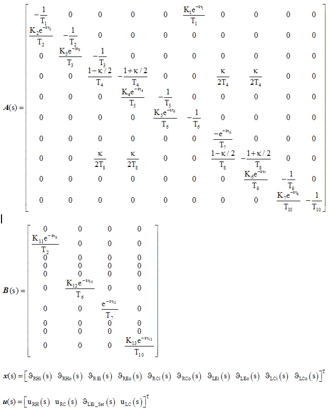
The first task solved in the thesis is to develop a model of the experimental heat transfer set-up. The linear model, which consists of ten functional differential equations describes the dynamics of the system in a vicinity of a selected operational point. All the state variables of the model represent temperatures measured at different places of the set-up. The model has four inputs which control the performance of the heaters and coolers respectively. The second, main task solved in the thesis is the control design of static gain coefficient feedback from the state variables by pole placement approaches. First the control design is solved as a SISO problem (a single system input is used for the control purpose and a single temperature is controlled) using both direct pole placement and continuous pole placement methods. Then the continuous pole placement method is used to design the feedback gains for DIDO problem (two system inputs are used for the control purpose and two temperatures are controlled). The resulting feedback controllers were successfully tested on the model as well as on the set-up. The control algorithms were implemented on both PC with Matlab and industrial PLC.

Experimental set-up consists of two independent heating circuits. Heat between circuits is transfered through the multiplate heat exchanger. Each heating circuit consists of: pump,mixing valve(s),pipe lines,cooler,heater. The scheme of heat system is shown in Fig.1 and photo in Fig.2.
The circulation of the medium in the circuit is forced by the Pump which is controlled manually by determining its pipe-lift. The flow through the pump is measured by a flow-meter. The heat source is an accumulation-type Heater. Notice that the inlet and the outlet water temperatures are measured as T_LHi and T_LHo , respectively. Even though the performance of the heater can be controlled by the signal U_LH, due to relatively large capacity of the heater, the control actions are slow. Therefore, it is better to control the water temperate which goes to the exchanger, and which is measured as T_LEi, by a mixing Valve, which is controlled by the signal U_LV1. In fact this signal, via a servo of the valve, controls the position of the valve seat determining the mixing ratio of the hot water from the heater and cooled water from the cooler. The temperature of the water leaving the exchanger in the left circuit is measured as T_LEo. The second mixing Valve in the left circuit, which is controlled by the signal U_LV2, allows us to divide the water stream into two branches. One of the braches goes to the exchanger and the other accomplishes a bypass of the exchanger. The flow through the bypass branch pipe is measured by a flow-rate-meter. In this way, by the signal U_LV2 we can control the amount of the heat transferred between the circuits. Consequently, the temperature of the water leaving the mixing valve and forced towards the Cooler is also determined by the mixing ratio in the valve given by U_LV2. The temperatures in the inlet and outlet of the Cooler are measured as T_LCi and T_LCo, respectively. The cooling performance is controlled by signal U_LC. The water which leaves the cooler is forced by the pump towards the Heater.
The circulation of the medium in the right circuit is forced by the Pump which is controlled manually by determining its pipe-lif. The flow through the pump is measured by a flow-rate-meter. The heat source is a flow-type Heater. Its inlet and the outlet water temperatures are measured as T_RHi and T_RHo, respectively. Unlike the dynamics of the Heater in the left circuit, the dynamics of this Heater is relatively fast and, therefore, the heater can serve well as an actuator controlling the water temperature entering the exchanger, which is measured as T_REi. Alternatively as an actuator by which this temperature can be controlled can serve the mixing Valve. In this valve, the hot water from the heater is mixed with cooled water from the Cooler R in a ratio determined by the position of the valve seat controlled via a servo by signal U_RV. This mixing valve determines the flow passing through the heater. The temperature of the water leaving the exchanger in the right circuit is measured as T_REo. The water is then forced towards the Cooler. Its inlet and outlet water temperatures are measured as T_RCi and T_RCo, respectively. The cooling performance is controlled by signal U_RC. The water which leaves the cooler is forced by the pump towards the Heater.

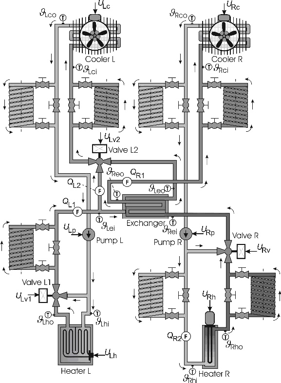
Fig.1 Scheme of the laboratory experimental set-up

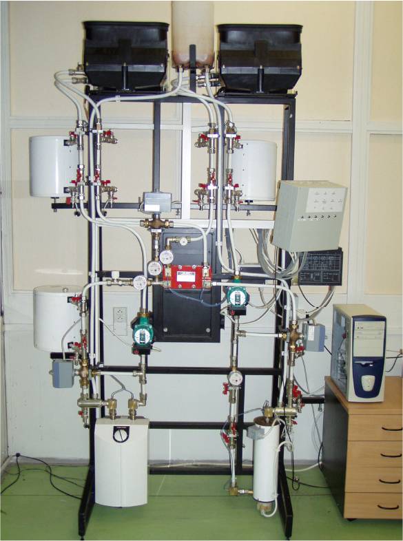
Fig. 2 Experimental set-up

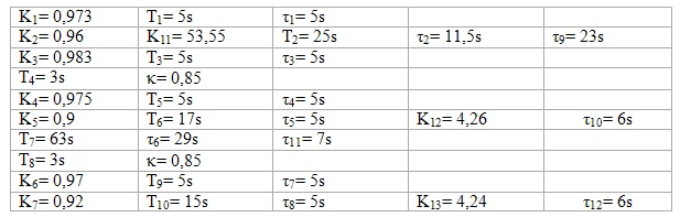
Model of the system consists of ten first order functional differential equations and may be written in form

sx(s) = A(s)x(s) + B(s)u(s)

where

Spectrum of this system is shown in Fig. 3. (quasipolynomial rootfinder was used, see [5])

Fig.3. Poles of thermal set-up

red contours - Im(M(s)) = 0; blue contours - Re(M(s)) = 0
M(s) = det[sI-A(s)]

Synthesis of state feedback controller (left circuit - SISO system)

We use a linear state feedback controller

u = - Kx(t)

The characteristic equations is as follows

M(s) = det[sI-A(s)+B(s)K]

Results achieved using direct pole placement method (see [1],[2]) are shown in Fig. 4

Fig.4. Poles of thermal set-up

Using continuous pole placement method (described in [3]) we obtain following results. In Fig.5 are shown poles of system, in Fig.6 and Fig.7 evolution of real parts of poles and coefficients.

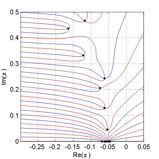
Fig.5. Poles of thermal set-up (left circuit)



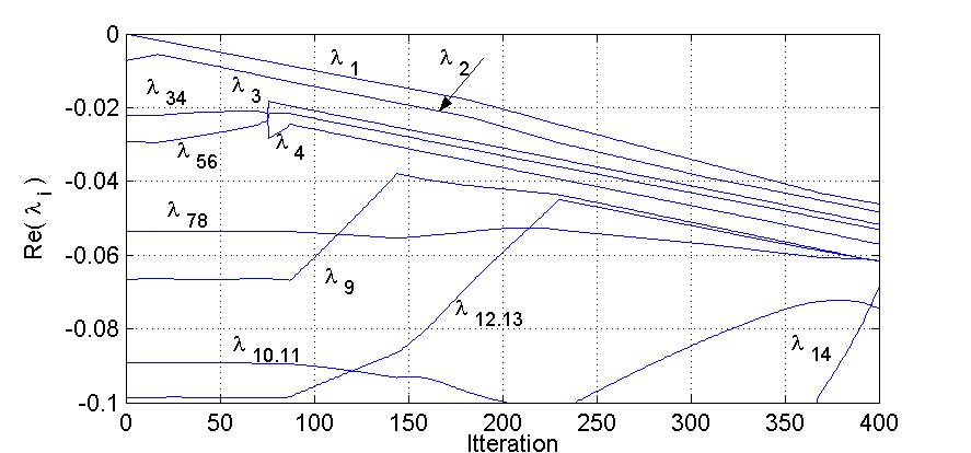
Fig.6. Evolution of real parts of system (left circuit)



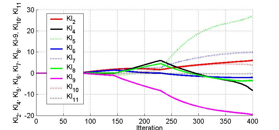
Fig.7. Evolution of coefficients(left circuit)

Simulations obtained using coefficients computed at different itterations are shown in Fig. 8. Step responses of system achived with use of coefficients from step 140 are shown in Fig.9.

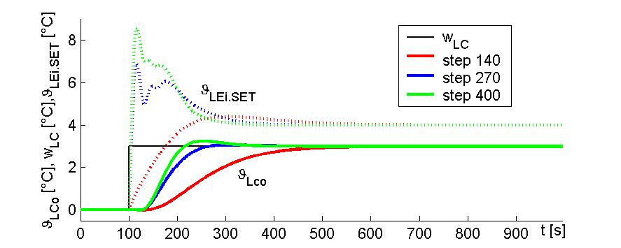
Fig.8. Simulations - Step responses (left circuit)

Coefficients computed in step 140:

KL1 = 0 , KL2 = 1,7463, KL3 = 0, KL4 = -0,1421, KL5 = -0,9795, KL6 = 1,3766, KL7 = 1,4114, KL8 = 0,436
KL9 = -1,0475, KL10 = -0,5405, KL11 = -0.0187

Coefficients computed in step 270:

KL1 = 0 , KL2 = 3,1265, KL3 = 0, KL4 = 1,8892, KL5 =13,1326, KL6 = -0,9987, KL7 = 5,7015, KL8 = 0,9220
KL9 =-13,4321, KL10 = 2,8531, KL11 = -0.1955

Coefficients computed in step 400:

KL1 = 0 , KL2 = 6.0359, KL3 = 0, KL4 = -8.1650, KL5 =26.9323, KL6 = -1.9985, KL7 = 9.8736, KL8 = -3.4711
KL9 -19.6151, KL10 = 3.7782, KL11 = -0.2519

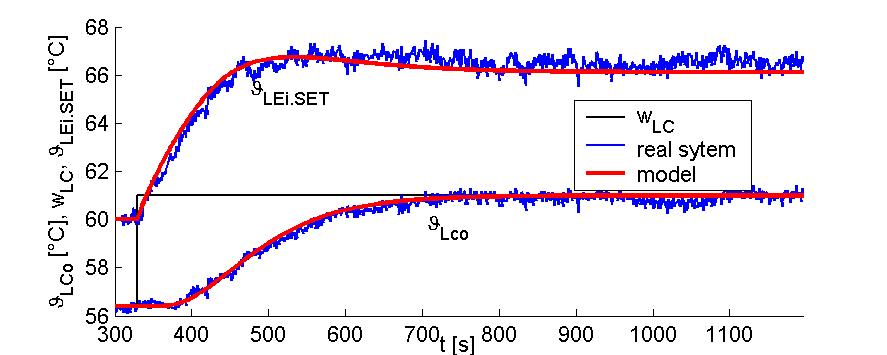
Fig.9. Step responses (left circuit) - Experimental thermal set-up

Synthesis of state feedback controller (MIMO system)

For MIMO system a coefficients of state feedback can not be computed using direct pole placement method (see [4]). Therefore only results of continuous pole placement will be presented - Fig.10, Fig.11., Fig.12

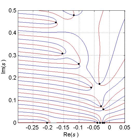
Fig.10. Poles of thermal set-up (MIMO system)



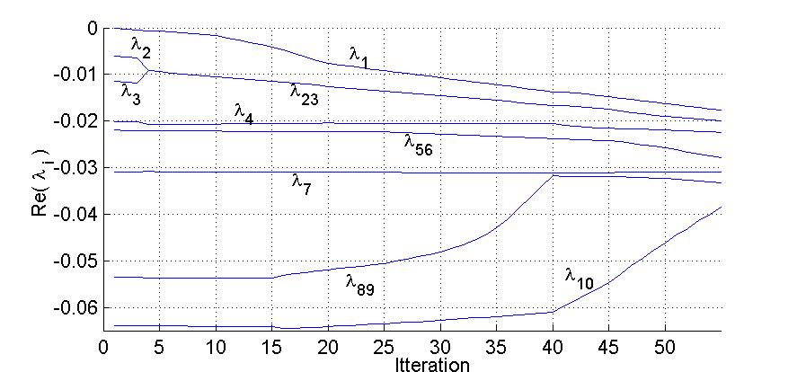
Fig.11. Evolution of real parts of system (MIMO system)



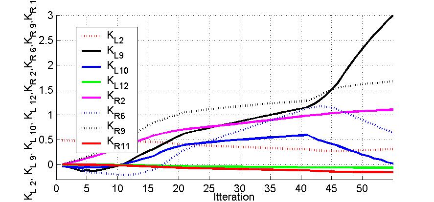
Fig.12. Evolution of coefficients (MIMO system)

Detailed results can be found in [4].

References

[1]  Zítek, P., Vyhlídal, T.: Dominant eigenvalue placement for time delay systems, In Proc. of Controlo, 5th Portuguese Conference on Automatic Control, University of Aveiro, Portugal, 2002

[2]  Vyhlídal,T.:Analysis and Synthesis of time delay systems spectrum, Ph.D.Thesis, CVUT, Faculty of Mechanical Engineering, 2003

[3]  Michiels, W., Engelborghs, K., Vansevenant, P., Roose, D.: Continuous pole placement for delay equations, Automatica, vol 38, no.6, pp. 747-761, 2002

[4]  Paulu, K.: Synthesis of control of experimental heat transfer set-up through state feedback, MSc Thesis (in czech), 2007

[5]  Vyhlidal, T., Zitek, P., Quasipolynomial mapping based rootfinder for analysis of time delay systems, In Proc. of IFAC Workshop on Time-Delay systems, Rocquencourt, 2003